}
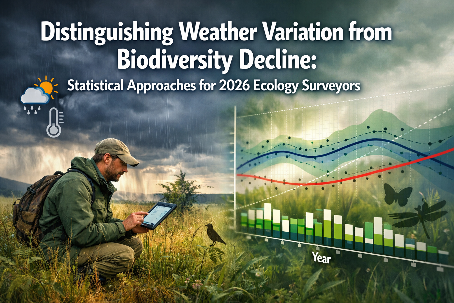
Weather-driven ecological variation can easily be mistaken for genuine biodiversity loss. A sudden drop in butterfly counts during an unusually cold spring, or a spike in amphibian observations following heavy rainfall, might suggest dramatic ecosystem changes that aren't actually occurring. For ecology surveyors working in 2026, the challenge of distinguishing weather variation from biodiversity decline has never been more critical—or more complex. With global wildlife populations having declined by approximately 69% since 1970, and climate patterns becoming increasingly erratic, separating short-term environmental noise from long-term ecological signals requires sophisticated statistical approaches and rigorous methodology.
This comprehensive guide explores the practical statistical methods that enable ecology surveyors to confidently distinguish weather variation from biodiversity decline, ensuring that monitoring data accurately reflects true ecosystem health rather than temporary environmental fluctuations.
Key Takeaways
- Weather-driven fluctuations can mask or mimic biodiversity trends, requiring multi-year baseline data and proper statistical controls to separate temporary variation from permanent decline
- Temporal stratification and standardized survey protocols across different weather conditions are essential for building robust datasets that account for environmental variability
- Advanced statistical methods including GAMs, hierarchical Bayesian models, and time-series decomposition provide powerful tools for distinguishing signal from noise in ecological monitoring data
- Integration of weather data directly into biodiversity analyses through covariates and interaction terms strengthens the reliability of trend assessments
- Proper baseline establishment typically requires 3-5 years of consistent monitoring before confident conclusions about biodiversity trends can be drawn
Understanding the Challenge: Why Weather Complicates Biodiversity Assessment
The Fundamental Problem for Ecology Surveyors
Ecological surveys capture snapshots of biodiversity at specific moments in time. However, species detectability, activity patterns, and apparent abundance can vary dramatically based on immediate weather conditions. A bird survey conducted during heavy rain will inevitably record fewer individuals than one performed during calm, clear weather—not because the population has declined, but because birds are less active and visible during precipitation.
This detectability problem extends across all taxonomic groups:
- 🦋 Invertebrates: Temperature, wind speed, and cloud cover directly affect flight activity and visibility
- 🐸 Amphibians: Rainfall patterns influence breeding behavior, migration, and calling activity
- 🌿 Plants: Seasonal weather variation affects flowering phenology and identification characteristics
- 🦅 Birds: Wind, temperature, and precipitation impact foraging behavior, vocalization, and movement patterns
- 🦎 Reptiles: Thermoregulation requirements make reptile activity highly weather-dependent
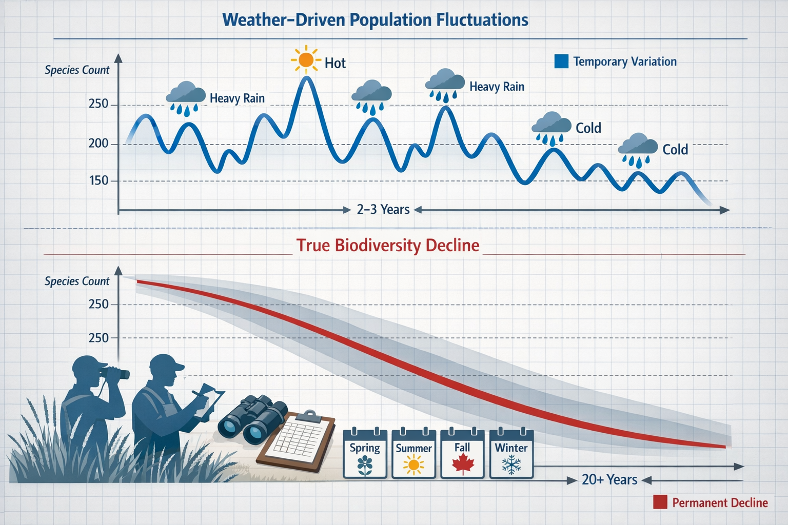
Short-Term Variation vs. Long-Term Trends
The critical distinction for surveyors lies between:
Weather-driven variation (reversible, temporary):
- Seasonal population fluctuations
- Migration timing shifts
- Breeding phenology changes
- Short-term resource availability
- Temporary habitat suitability changes
Biodiversity decline (directional, persistent):
- Habitat loss and fragmentation
- Pollution and contamination
- Invasive species establishment
- Climate change impacts
- Disease emergence
Without proper analytical frameworks, even experienced surveyors can misinterpret temporary weather-related changes as evidence of biodiversity trends. This confusion can lead to inappropriate management decisions, wasted conservation resources, or—equally problematic—failure to detect genuine declines requiring urgent intervention.
Statistical Approaches for Distinguishing Weather Variation from Biodiversity Decline
Establishing Robust Baseline Data
The foundation of distinguishing weather variation from biodiversity decline begins with proper baseline establishment. Single-year surveys, regardless of statistical sophistication, cannot reliably separate temporary fluctuations from directional trends.
Minimum baseline requirements:
| Survey Objective | Minimum Duration | Recommended Duration | Survey Frequency |
|---|---|---|---|
| Trend detection | 3 years | 5+ years | Seasonal (quarterly) |
| Impact assessment | 2 years pre-impact | 3+ years pre-impact | Monthly |
| Habitat comparison | 1 year | 2+ years | Seasonal |
| Rare species monitoring | 3 years | 5+ years | Species-specific |
Baseline data should encompass diverse weather conditions to capture the full range of natural variation. Surveys conducted only during optimal weather will create biased baselines that make normal variation appear as decline when less favorable conditions occur.
Temporal Stratification and Standardization
Temporal stratification involves organizing survey effort across time periods to ensure comparable data collection. For ecology surveyors implementing biodiversity impact assessments, this means:
- Fixed survey windows: Conducting surveys during the same phenological periods each year (e.g., "third week of May" rather than "when weather is optimal")
- Consistent timing: Maintaining similar time-of-day schedules to control for diurnal activity patterns
- Weather documentation: Recording detailed weather parameters during each survey (temperature, precipitation, wind speed, cloud cover, humidity)
- Effort standardization: Maintaining consistent survey duration, observer numbers, and spatial coverage
This standardization creates datasets where weather becomes a documented variable rather than an uncontrolled confounding factor.
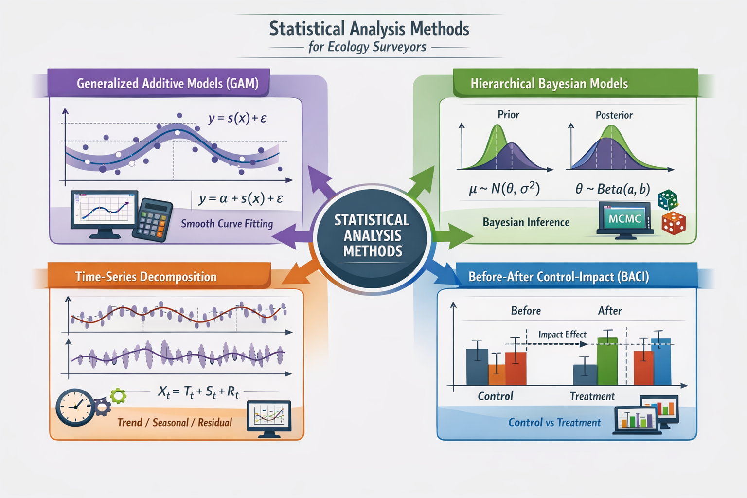
Generalized Additive Models (GAMs)
Generalized Additive Models provide flexible frameworks for modeling non-linear relationships between biodiversity metrics and environmental variables. For distinguishing weather variation from biodiversity decline, GAMs excel at:
- Fitting smooth curves to temporal trends without assuming linear relationships
- Incorporating weather covariates as smooth functions
- Handling non-normal distributions common in count data
- Separating long-term trends from seasonal patterns
Practical GAM application:
Species_Count ~ s(Year, k=5) + s(Day_of_Year, bs="cc") +
                s(Temperature) + s(Precipitation) +
                Habitat_Type + Observer
This model structure separates:
- Long-term trend (
s(Year)) - Seasonal variation (
s(Day_of_Year)) - Weather effects (
s(Temperature),s(Precipitation)) - Habitat and observer differences
The year effect represents the biodiversity trend after accounting for weather-driven variation, providing the clearest signal of actual population change.
Hierarchical Bayesian Models
Hierarchical Bayesian approaches offer powerful advantages for ecology surveyors working with limited data or complex nested structures. These models explicitly separate:
- Process variation: True biological changes in populations
- Observation variation: Measurement error and detectability issues
- Environmental variation: Weather and habitat effects
For 2026 ecology surveyors, hierarchical models enable:
✅ Incorporation of prior knowledge from similar ecosystems or species
✅ Explicit uncertainty quantification through posterior distributions
✅ Missing data handling without losing entire survey periods
✅ Multi-level structure accounting for sites nested within regions, surveys nested within years
These models produce credible intervals that honestly represent uncertainty, helping surveyors communicate confidence levels when distinguishing weather variation from biodiversity decline.
Time-Series Decomposition Methods
Time-series decomposition breaks observed biodiversity data into interpretable components:
- Trend component: Long-term directional change (the biodiversity signal)
- Seasonal component: Predictable within-year variation (phenology)
- Weather component: Short-term environmental effects
- Residual component: Unexplained random variation
Classical decomposition methods (additive or multiplicative) provide intuitive visualizations, while more sophisticated approaches like STL (Seasonal and Trend decomposition using Loess) handle complex patterns and missing data.
For ecology surveyors, decomposition reveals whether apparent changes represent:
- 📈 Genuine trends requiring management response
- 🔄 Cyclical patterns requiring longer monitoring
- ☁️ Weather-driven noise requiring statistical control
Before-After-Control-Impact (BACI) Designs
When assessing biodiversity changes related to specific events or interventions, BACI designs provide robust frameworks for distinguishing weather variation from biodiversity decline. This approach compares:
- Before and After the event/intervention
- Control sites (unaffected) and Impact sites (affected)
The key advantage: weather affects both control and impact sites similarly, so differences between them reflect genuine biodiversity changes rather than environmental variation.
Statistical implementation:
Biodiversity_Metric ~ Period (Before/After) × Location (Control/Impact) +
                      Weather_Covariates + Random_Effects
The interaction term (Period × Location) isolates the true impact from weather-driven changes affecting all sites. This design proves particularly valuable for biodiversity net gain assessments where development impacts must be distinguished from background variation.
Integrating Weather Data into Biodiversity Analysis
Essential Weather Variables for Ecology Surveyors
Effective integration of weather data requires collecting relevant meteorological parameters during each survey:
Primary weather variables:
- 🌡️ Temperature: Air temperature at survey time (°C)
- 💧 Precipitation: Recent rainfall (24-hour, 7-day, 30-day totals)
- 💨 Wind speed: Current wind conditions (m/s or Beaufort scale)
- ☁️ Cloud cover: Percentage or categorical (clear/partly cloudy/overcast)
- 💦 Humidity: Relative humidity percentage
- 🌅 Light conditions: Time since sunrise/until sunset
Secondary variables (species-specific):
- Soil moisture (for soil-dwelling invertebrates)
- Water temperature (for aquatic species)
- Snow depth (for winter surveys)
- Barometric pressure (for some insect groups)
Weather Data Sources and Integration
Modern ecology surveyors in 2026 have access to multiple weather data sources:
- On-site measurements: Portable weather stations provide precise local conditions
- Nearby weather stations: Government meteorological services offer historical data
- Gridded climate datasets: Spatial interpolation provides site-specific estimates
- Remote sensing: Satellite data for temperature, precipitation, and vegetation indices
Best practice: Combine on-site measurements during surveys with historical weather station data to capture both immediate conditions and longer-term weather patterns (e.g., cumulative rainfall over preceding weeks).
Lagged Weather Effects
Many biodiversity responses to weather involve time lags. For example:
- Butterfly abundance may depend on temperature 2-3 weeks prior (affecting larval development)
- Amphibian breeding activity relates to rainfall patterns over the previous month
- Plant flowering responds to accumulated degree-days over weeks or months
Incorporating lagged weather variables into statistical models captures these delayed responses:
Species_Abundance ~ Temperature_Current +
                    Temperature_Lag_2weeks +
                    Precipitation_30day +
                    Year_Trend
This approach prevents misattributing lagged weather effects to biodiversity trends.
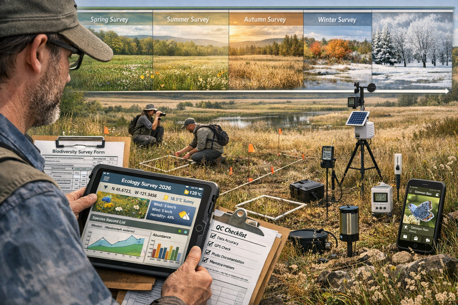
Practical Implementation for 2026 Ecology Surveyors
Survey Protocol Design
Robust protocols for distinguishing weather variation from biodiversity decline incorporate:
1. Standardized survey conditions
- Define acceptable weather ranges (e.g., "surveys conducted when temperature >12°C, wind <5m/s, no heavy precipitation")
- Document all deviations from standard conditions
- Avoid systematically surveying only during optimal weather
2. Replicate surveys
- Conduct multiple surveys per season to capture weather variation
- Space surveys to encompass different weather conditions
- Maintain consistent spatial coverage across survey occasions
3. Weather documentation
- Record weather parameters at survey start, middle, and end
- Note weather changes during survey period
- Photograph conditions for qualitative reference
4. Observer consistency
- Maintain consistent observer teams where possible
- Conduct inter-observer calibration exercises
- Include observer identity as random effect in analyses
These protocols support biodiversity net gain planning by ensuring baseline and post-development monitoring data remain comparable despite weather variation.
Data Management and Quality Control
Quality control procedures essential for distinguishing weather variation from biodiversity decline:
✔️ Real-time data validation: Check for obvious errors during field work
✔️ Weather data verification: Cross-reference on-site measurements with nearby stations
✔️ Outlier investigation: Examine extreme values for data entry errors vs. genuine observations
✔️ Metadata documentation: Record equipment calibration, observer changes, protocol modifications
✔️ Spatial accuracy: Verify GPS coordinates and habitat classifications
Robust data management ensures that apparent biodiversity changes reflect ecological reality rather than data quality issues.
Analytical Workflows
Step-by-step workflow for distinguishing weather variation from biodiversity decline:
Phase 1: Exploratory Analysis
- Visualize raw data across time (time-series plots)
- Examine distributions and identify outliers
- Assess correlations between biodiversity metrics and weather variables
- Check for obvious seasonal patterns
Phase 2: Model Development
- Fit baseline models without weather covariates
- Add weather variables and compare model fit
- Test for interactions between weather and time
- Validate models using held-out data or cross-validation
Phase 3: Trend Assessment
- Extract year effects from best-fitting models
- Calculate confidence intervals for trends
- Assess whether trends differ significantly from zero
- Quantify proportion of variation explained by weather vs. trend
Phase 4: Interpretation
- Compare statistical trends to biological expectations
- Consider alternative explanations for patterns
- Assess whether trends warrant management action
- Identify data gaps requiring additional monitoring
This systematic approach ensures rigorous distinction between weather-driven variation and genuine biodiversity change, supporting evidence-based conservation decisions and achieving biodiversity net gain objectives.
Software Tools and Resources
Modern ecology surveyors have access to powerful analytical tools:
Statistical software:
- R: Free, open-source with extensive ecological packages (mgcv, unmarked, jagsUI)
- Python: Flexible programming with scientific libraries (statsmodels, PyMC3)
- JAGS/Stan: Specialized Bayesian inference platforms
- TRIM: Dedicated software for trend analysis in monitoring data
Key R packages for weather-biodiversity analysis:
mgcv: Generalized additive modelslme4/nlme: Mixed-effects modelsbsts: Bayesian structural time-seriesforecast: Time-series decompositionunmarked: Occupancy and abundance modeling accounting for detectability
Data repositories:
- Weather data: National meteorological services, NOAA, ERA5 reanalysis
- Biodiversity data: NBN Atlas, GBIF, local biological records centers
Common Pitfalls and How to Avoid Them
Insufficient Baseline Data
Problem: Drawing conclusions from single-year surveys or short monitoring periods.
Solution: Commit to multi-year monitoring programs (minimum 3 years) before making definitive trend assessments. Communicate uncertainty honestly when baseline data remain limited.
Confounding Weather with Phenology
Problem: Attributing seasonal variation to weather effects or vice versa.
Solution: Include both seasonal terms (day of year, month) and weather variables in models to separate these effects.
Ignoring Detectability
Problem: Treating observed counts as true abundance without accounting for detection probability.
Solution: Implement occupancy models, distance sampling, or repeated surveys that explicitly estimate and correct for imperfect detection.
Overfitting Statistical Models
Problem: Including too many weather variables or overly complex smooth functions, causing models to fit noise rather than signal.
Solution: Use model selection criteria (AIC, BIC) and cross-validation to identify parsimonious models. Prioritize biological plausibility over statistical fit.
Weather Station Distance
Problem: Using weather data from distant stations that don't represent local site conditions.
Solution: Verify that weather stations are within appropriate distance (<10km for most variables) and similar elevation/topography. Validate with on-site measurements.
Publication Bias
Problem: Focusing only on statistically significant trends while ignoring stable populations.
Solution: Report all findings, including non-significant trends and stable populations. Absence of decline is valuable information for biodiversity net gain monitoring.
Case Study Applications
Example 1: Grassland Butterfly Monitoring
A five-year butterfly transect survey showed apparent 40% decline in total abundance. However, statistical analysis revealed:
- Weather effects: Temperature and wind speed explained 65% of variation
- Trend after weather correction: Non-significant 8% decline (confidence interval: -22% to +9%)
- Conclusion: Observed decline primarily reflected weather variation, particularly cooler summers in years 3-4
Key lesson: Weather-corrected analysis prevented unnecessary habitat management interventions.
Example 2: Amphibian Breeding Assessment
Pond surveys detected 60% reduction in breeding amphibians over three years, raising conservation concerns. Detailed analysis showed:
- Precipitation patterns: Drought conditions in year 2 reduced breeding activity
- BACI comparison: Control ponds showed similar patterns
- Recovery: Year 4 monitoring (normal rainfall) showed population recovery
- Conclusion: Temporary weather-driven breeding suppression, not population decline
Key lesson: Extended monitoring through varied weather conditions revealed resilience rather than decline.
Future Directions for Ecology Surveyors in 2026
Emerging Technologies
Automated monitoring systems increasingly supplement traditional surveys:
- 🎤 Acoustic monitoring: Continuous recording captures species activity across weather conditions
- 📷 Camera traps: 24/7 monitoring reduces weather-related survey bias
- 🛰️ Remote sensing: Satellite imagery tracks habitat changes independent of ground weather
- 🤖 AI identification: Machine learning processes large datasets, identifying weather-abundance relationships
These technologies generate vast datasets that demand sophisticated statistical approaches for distinguishing weather variation from biodiversity decline.
Climate Change Considerations
As climate patterns shift, the distinction between weather variation and biodiversity decline becomes increasingly nuanced. Novel climate conditions may represent:
- Temporary extreme weather events (variation)
- Permanent climate regime shifts (decline drivers)
- Transitional periods requiring adaptive management
Ecology surveyors must consider whether observed weather patterns represent:
- Natural variability within historical ranges
- New climate normals requiring baseline adjustment
- Directional climate trends affecting biodiversity directly
Integration with Biodiversity Net Gain
For surveyors supporting biodiversity net gain requirements, distinguishing weather variation from biodiversity decline ensures:
- Accurate baseline assessments not biased by weather during survey periods
- Reliable impact predictions based on genuine trends rather than fluctuations
- Effective monitoring that detects real changes requiring adaptive management
- Credible reporting supporting regulatory compliance and conservation outcomes
Statistical rigor in separating signal from noise strengthens the entire biodiversity net gain framework, ensuring development impacts are properly assessed and mitigated.
Conclusion
Distinguishing weather variation from biodiversity decline represents one of the most critical challenges facing ecology surveyors in 2026. With wildlife populations facing unprecedented pressures and climate patterns becoming increasingly variable, the ability to separate short-term environmental noise from genuine ecological signals has never been more important.
The statistical approaches outlined in this guide—from generalized additive models and hierarchical Bayesian frameworks to time-series decomposition and BACI designs—provide powerful tools for making this essential distinction. However, these methods succeed only when built upon robust baseline data, standardized protocols, and comprehensive weather documentation.
Actionable Next Steps for Ecology Surveyors
- Evaluate current protocols: Assess whether existing survey designs adequately document weather conditions and encompass sufficient temporal replication
- Establish multi-year baselines: Commit to monitoring programs spanning at least 3-5 years before drawing definitive conclusions about biodiversity trends
- Integrate weather data: Systematically collect and incorporate meteorological parameters into all biodiversity analyses
- Adopt appropriate statistical methods: Select analytical approaches that explicitly separate weather effects from temporal trends
- Invest in training: Develop statistical literacy in GAMs, Bayesian methods, and time-series analysis
- Collaborate with specialists: Partner with statisticians and climatologists for complex analyses
- Communicate uncertainty: Honestly report confidence intervals and limitations when distinguishing variation from decline
By implementing these approaches, ecology surveyors can provide the rigorous, defensible evidence needed to guide conservation decisions, support biodiversity net gain objectives, and ensure that management interventions address genuine biodiversity declines rather than temporary weather-driven fluctuations.
The stakes are high: misinterpreting weather variation as decline wastes limited conservation resources, while failing to detect genuine declines allows irreversible biodiversity loss. Statistical rigor in distinguishing these patterns represents not just methodological best practice, but an ethical imperative for ecology professionals committed to evidence-based conservation in an era of unprecedented environmental change.