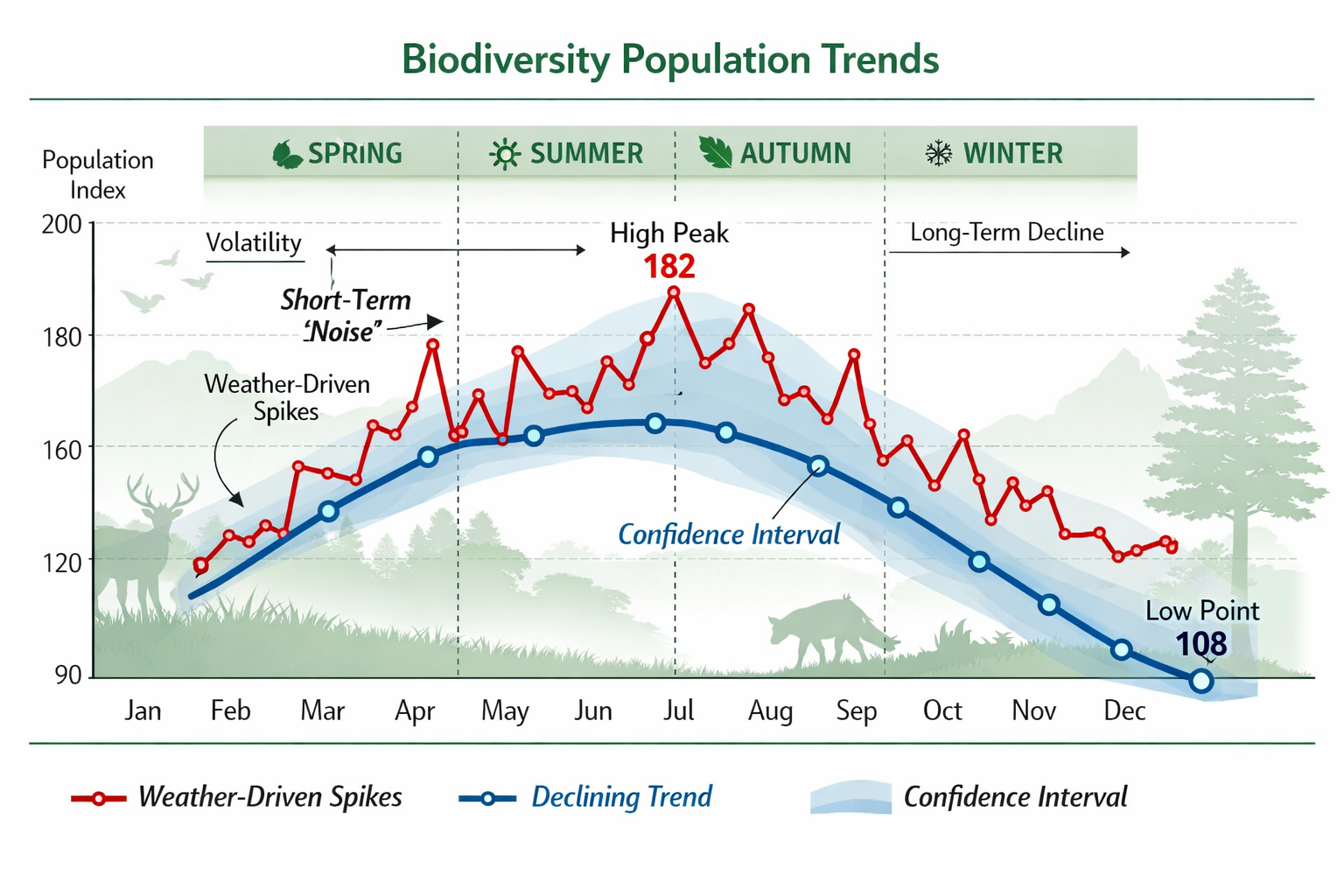
A sudden drop in bird populations appears in your spring survey. Is this the beginning of a long-term decline requiring urgent intervention? Or simply a cold snap that delayed migration by two weeks? Without continuous monitoring, these scenarios look identical—yet they demand completely different responses. As biodiversity loss accelerates globally, the ability to separate genuine ecological decline from natural weather-driven variation has become critical for effective conservation in 2026.
Weather-driven variation can masquerade as population decline in snapshot surveys, leading to misallocated resources and ineffective interventions. Meanwhile, true biodiversity trends remain hidden beneath seasonal fluctuations and short-term disturbances. This challenge affects everyone from developers implementing Biodiversity Net Gain strategies to conservation scientists tracking endangered species.
The solution lies in continuous monitoring strategies combined with robust statistical frameworks that reveal patterns invisible to one-off surveys. This approach transforms how we understand ecosystem health, enabling data-driven decisions that distinguish real ecological signals from environmental noise.
Key Takeaways
- 🔍 Weather-driven variation mimics long-term decline in single-point surveys, creating false signals that can mislead conservation efforts without continuous data collection
- 📊 Statistical frameworks using Bayesian models can separate true population trends from natural variation by accounting for spatial and temporal autocorrelation across thousands of time series
- 🌱 Full-season monitoring starting in early spring captures the complete arc of biological activity, establishing baselines strong enough to detect intervention effectiveness
- 🤖 Emerging technologies like TinyML and satellite-AI fusion enable real-time biodiversity detection in remote landscapes, revolutionizing continuous monitoring capabilities in 2026
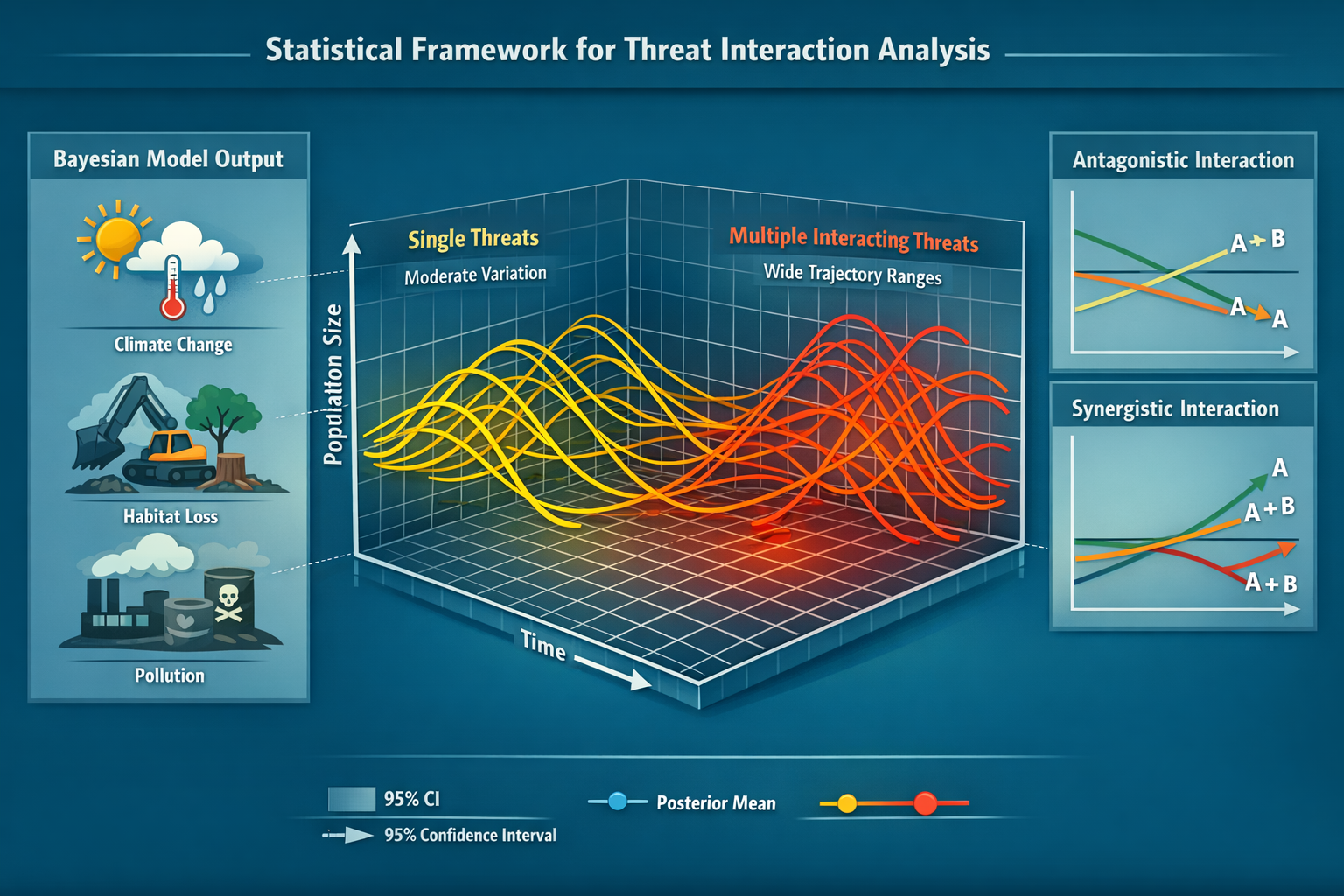
- ⚠️ Multiple interacting threats show wider trajectory ranges than single threats, with antagonistic interactions predominating at population levels—requiring continuous data to detect and understand
Understanding the Signal-Noise Problem in Biodiversity Assessment
The Fundamental Challenge
Biodiversity data contains two types of information: signal (genuine long-term trends) and noise (short-term fluctuations). Weather events, seasonal cycles, and temporary disturbances create variation that can completely obscure underlying population trajectories. A comprehensive analysis of 3,129 vertebrate population time series worldwide revealed that without proper statistical controls for spatial and temporal autocorrelation, these patterns blur together[3].
The consequences are significant. Conservation interventions can appear effective or ineffective simply because baseline data lacks the strength to separate signal from noise[2]. Resources flow toward false alarms while genuine declines go undetected. For developers working on biodiversity impact assessments, this uncertainty creates compliance risks and planning delays.
Why One-Off Surveys Fall Short
Traditional biodiversity surveys provide detailed snapshots—species counts, habitat conditions, community composition at a single point in time. These assessments serve important purposes, particularly for regulatory compliance and initial site characterization. However, they cannot capture:
- Seasonal dynamics that shift species abundance by orders of magnitude
- Weather-driven population fluctuations that reverse within weeks
- Delayed responses to habitat changes that emerge over multiple years
- Recovery trajectories following disturbance events
- Baseline variability necessary to detect statistically significant trends
Without continuous, multi-season monitoring, weather-driven variation can be mistaken for long-term decline, while short-term disturbances may look like recovery[2]. The timing of a single survey can determine whether a site appears species-rich or species-poor, regardless of its actual ecological value.
The Cost of Misinterpretation
Misreading biodiversity signals carries real consequences:
False positives trigger unnecessary interventions, wasting limited conservation budgets on populations that would naturally rebound. False negatives allow genuine declines to continue undetected until recovery becomes impossible. Incorrect baselines make it impossible to demonstrate whether management actions achieve their intended outcomes.
For landowners considering selling biodiversity units or developers planning how to achieve 10% Biodiversity Net Gain, these uncertainties create financial and regulatory risks that continuous monitoring can mitigate.
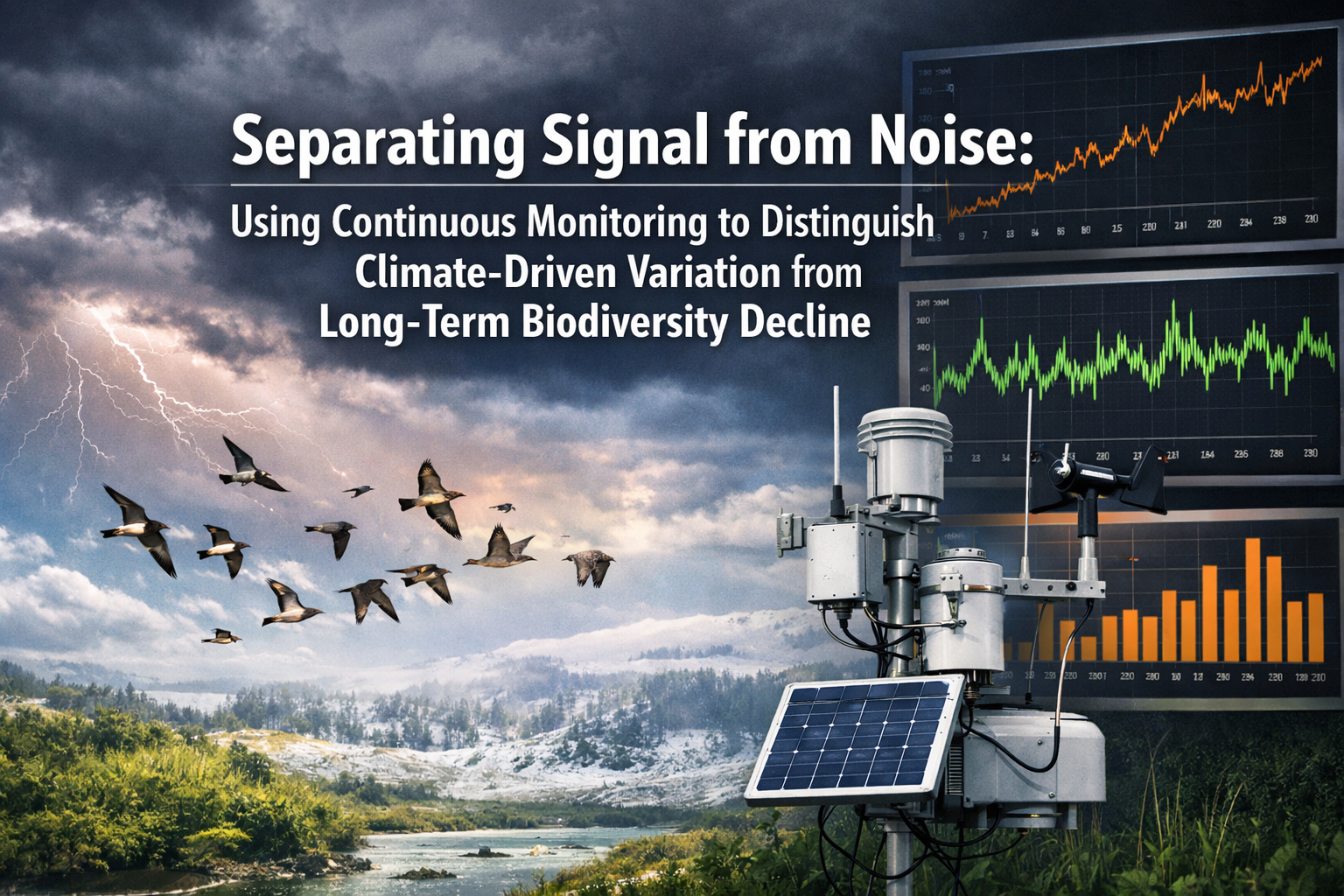
Separating Signal from Noise: Using Continuous Monitoring to Distinguish Climate-Driven Variation from Long-Term Biodiversity Decline Through Data Collection
Establishing Robust Baselines
Continuous monitoring reveals patterns, trends, and anomalies that static assessments miss[2]. The key lies in establishing baselines early and maintaining consistent data collection across full biological cycles. Beginning monitoring in early spring allows capture of the complete arc of biological activity—from first emergence through peak summer activity and into seasonal decline[2].
This timing matters profoundly. Starting in April means datasets reflect the ecosystem's rhythm, not just its peak[2]. A monitoring program that begins in June will systematically underestimate spring-breeding species, overweight summer residents, and miss early-season phenological shifts that signal climate impacts.
Frequency and Duration Requirements
Effective continuous monitoring requires strategic decisions about:
Sampling frequency: Weekly to monthly observations capture seasonal patterns while remaining cost-effective. More frequent sampling may be necessary during critical periods (breeding seasons, migration windows) or when detecting rapid changes.
Monitoring duration: Minimum 2-3 years to distinguish annual variation from directional trends. Ideally 5+ years to detect responses to management interventions with statistical confidence.
Seasonal coverage: Full-year monitoring captures all life stages and seasonal visitors. Partial-year programs should align with target species' activity periods and maintain consistent timing across years.
Spatial replication: Multiple monitoring points within sites reveal spatial heterogeneity and strengthen statistical inference about site-level trends.
Multi-Taxa Approaches
Comprehensive biodiversity monitoring extends beyond single species or taxonomic groups. Multi-taxa approaches provide:
- Cross-validation of trends across different organisms with varying life histories
- Early warning signals from taxa with rapid response times to environmental change
- Ecosystem-level insights impossible to obtain from single-species monitoring
- Efficiency gains through coordinated field efforts capturing multiple groups simultaneously
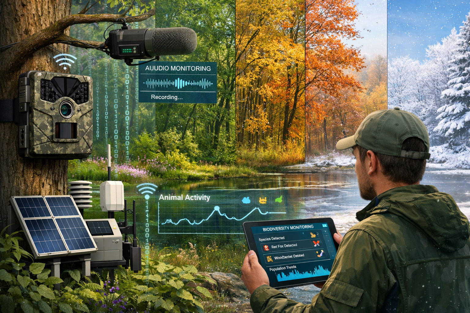
Modern technologies enable simultaneous monitoring of birds (acoustic recorders), insects (camera traps with AI identification), plants (repeat photography), and mammals (motion-triggered cameras) from single field deployments.
Integrating Environmental Covariates
Separating signal from noise requires measuring the noise itself. Continuous monitoring programs should incorporate:
- Weather data: Temperature, precipitation, wind patterns affecting species activity and detectability
- Phenological markers: Vegetation green-up, flowering timing, leaf fall indicating seasonal progression
- Habitat conditions: Water levels, vegetation structure, disturbance events
- Human activities: Management interventions, adjacent land use changes, visitor pressure
These covariates enable statistical models to attribute variation to specific drivers rather than treating all fluctuation as unexplained noise.
Statistical Frameworks for Distinguishing True Trends from Natural Variation
Bayesian Hierarchical Models
The most powerful approach for separating signal from noise in biodiversity data employs multilevel Bayesian models that explicitly account for multiple sources of variation[3]. These frameworks partition observed changes into:
- Fixed effects: Systematic trends attributable to specific threats or interventions
- Random effects: Site-specific and temporal variation not explained by measured predictors
- Spatial autocorrelation: Non-independence of nearby populations
- Temporal autocorrelation: Carryover effects from previous time periods
A global analysis of vertebrate populations used this approach to demonstrate that interactive threats are associated with stronger declines than random effects—meaning threat interactions produce real ecological signals distinct from natural variation[3]. This finding would be impossible to detect without statistical methods that explicitly separate different variance components.
Handling Autocorrelation
Biodiversity time series violate standard statistical assumptions because observations are not independent. Temporal autocorrelation means this year's population depends partly on last year's. Spatial autocorrelation means nearby sites share unmeasured environmental drivers.
Ignoring these dependencies inflates apparent sample sizes and produces false confidence in trends. Proper models incorporate:
- Autoregressive terms capturing temporal dependencies
- Spatial random effects accounting for geographic structure
- Phylogenetic controls for taxonomic non-independence when analyzing multiple species
Detecting Threshold Effects and Regime Shifts
Not all ecological change is gradual. Threshold effects occur when systems shift abruptly between states once environmental conditions cross critical values. Continuous monitoring enables detection of:
- Early warning signals: Increased variance and autocorrelation preceding regime shifts
- Tipping points: Rapid non-linear responses to gradual environmental change
- Hysteresis: Different trajectories during decline versus recovery
These patterns remain invisible in snapshot surveys but become apparent with sufficient temporal resolution.
Quantifying Uncertainty
Effective decision-making requires knowing not just whether populations are declining, but how confident we are in that assessment. Bayesian frameworks naturally produce:
- Credible intervals: Ranges containing the true trend with specified probability
- Probability of decline: Direct statements like "85% probability this population is declining"
- Power analysis: Assessment of whether monitoring duration and intensity can detect biologically meaningful changes
This explicit uncertainty quantification enables risk-based decision-making for conservation and development planning, particularly relevant for biodiversity net gain assessments requiring defensible evidence.
Emerging Technologies Revolutionizing Continuous Monitoring in 2026
Tiny Machine Learning for Remote Detection
The 2026 Global Horizon Scan identifies Tiny Machine Learning (TinyML) as a transformative technology for biodiversity monitoring[1]. These low-power devices perform AI-based species identification without internet connectivity, enabling:
- Real-time detection in remote landscapes previously inaccessible to continuous monitoring
- Minimal energy requirements allowing years of autonomous operation on small batteries or solar panels
- Edge processing that analyzes data on-device, transmitting only detection events rather than raw sensor data
- Cost reductions making continuous monitoring economically feasible at landscape scales
Optical AI chips requiring minimal energy further enhance these capabilities, potentially enabling networks of thousands of monitoring points across conservation areas and development sites[1].
Earth Observation and Satellite-AI Fusion
The fusion of Earth observation and AI is reshaping biodiversity research by enabling predictive modeling and real-time monitoring[4]. Since 1972, the Landsat programme has provided one of the longest continuous global records of Earth's surface, enabling scientists to detect shifts in ecosystems too large or remote for traditional field surveys[4].
Modern applications combine:
- Multi-spectral satellite imagery capturing vegetation health, water availability, and habitat structure
- Machine learning algorithms identifying habitat types and detecting changes at pixel-level resolution
- Time-series analysis revealing seasonal patterns and long-term trajectories
- Validation networks linking satellite signals to ground-based biodiversity data
This technology enables continuous monitoring of habitat quality across entire landscapes, providing context for site-specific field surveys and early warning of large-scale changes.
Acoustic and Camera Trap Networks
Automated recording devices have matured into reliable, cost-effective monitoring tools:
Acoustic monitoring captures vocalizing species (birds, amphibians, bats, insects) continuously, with AI algorithms identifying species from sound recordings. Networks of recorders provide temporal and spatial coverage impossible with human observers.
Camera traps with AI-powered image recognition detect mammals and ground-dwelling birds 24/7, recording behavior, abundance, and phenology without human presence effects.
These technologies generate massive datasets requiring robust data management and analysis pipelines, but provide unprecedented insight into ecosystem dynamics.
Integration with Biodiversity Net Gain Monitoring
For developers and landowners engaged in Biodiversity Net Gain delivery, these technologies offer practical solutions for 30-year monitoring requirements. Automated systems can:
- Document baseline conditions before development
- Track habitat creation and enhancement progress
- Verify achievement of target conditions
- Provide auditable evidence for regulatory compliance
- Reduce long-term monitoring costs compared to repeated manual surveys
Real-World Applications: Separating Signal from Noise in Practice
Case Study: Multiple Threat Interactions
A comprehensive analysis of 3,129 vertebrate population time series revealed that populations facing multiple interacting threats displayed a much wider range of trajectories than those facing single threats, showing both the most positive and negative trends[3]. This pattern would appear as simple "noise" in snapshot assessments.
Critically, the predominance of antagonisms contrasts with conclusions drawn from meta-analyses of experimental systems, which generally report synergies as the dominant form of nonadditive interaction[3]. This discrepancy highlights how continuous population-level monitoring reveals dynamics invisible in short-term experiments.
Weather-Driven Variation Masking Trends
Consider a wetland bird population monitored monthly over three years. Year one shows high abundance during a wet spring. Year two shows 40% decline during drought. Year three shows partial recovery with normal rainfall. A single survey in year two would suggest severe decline requiring intervention. Continuous monitoring reveals a population tracking rainfall variation around a stable long-term mean—no intervention needed, but continued observation essential.
Detecting Intervention Effectiveness
A habitat restoration project aims to increase pollinator abundance. Post-restoration surveys show variable results—some months higher than baseline, others lower. Without continuous pre-restoration monitoring establishing natural variation, it's impossible to determine whether the intervention succeeded. With multi-year baseline data and continued post-restoration monitoring, statistical models can detect whether abundance increases exceed natural variation with quantifiable confidence.
This principle applies directly to creating biodiversity plans for development projects, where demonstrating net gain requires proving enhancement exceeds what would occur naturally.
Practical Implementation for Conservation and Development
Designing Effective Monitoring Programs
Successful continuous monitoring requires:
-
Clear objectives: What specific questions must the monitoring answer? What level of change must be detected?
-
Appropriate methods: Match monitoring techniques to target taxa, habitats, and resources available
-
Statistical power analysis: Ensure sampling intensity and duration can detect meaningful changes
-
Quality control protocols: Standardize methods across observers and time periods to minimize non-ecological variation
-
Data management systems: Establish workflows for data collection, storage, quality checking, and analysis
-
Adaptive frameworks: Build in periodic review and adjustment based on emerging results
Cost-Benefit Considerations
Continuous monitoring requires greater upfront investment than one-off surveys, but provides:
- Reduced long-term costs through early detection of problems before expensive interventions become necessary
- Regulatory certainty with defensible evidence for compliance with Biodiversity Net Gain requirements
- Optimized management by identifying which interventions actually work
- Risk mitigation by distinguishing genuine declines from natural variation
For development projects, integrating continuous monitoring from initial baseline through construction and post-completion phases creates a seamless evidence chain demonstrating environmental responsibility.
Collaboration and Data Sharing
Maximum value emerges when monitoring data contributes to broader understanding:
- Regional networks reveal landscape-scale patterns invisible at site level
- Cross-project comparisons identify general principles versus site-specific responses
- Open data initiatives enable meta-analyses detecting global patterns
- Stakeholder engagement builds support for conservation through transparent evidence
Conclusion
Separating signal from noise: using continuous monitoring to distinguish climate-driven variation from long-term biodiversity decline represents one of the most critical challenges facing conservation and sustainable development in 2026. Weather-driven fluctuations, seasonal cycles, and short-term disturbances create variation that can completely obscure genuine ecological trends in snapshot surveys. Without continuous data collection and robust statistical frameworks, resources flow toward false alarms while real declines go undetected.
The solution combines strategic monitoring design that captures full seasonal cycles with Bayesian statistical approaches that explicitly partition variation into signal and noise components. Emerging technologies—from TinyML devices enabling real-time species detection to satellite-AI fusion revealing landscape-scale patterns—make continuous monitoring increasingly feasible and cost-effective.
For conservation practitioners, the message is clear: establish baselines early, maintain consistent monitoring through complete biological cycles, and employ statistical methods that account for autocorrelation and environmental covariates. For developers and landowners engaged in Biodiversity Net Gain, continuous monitoring transforms from regulatory burden to strategic advantage, providing defensible evidence of environmental outcomes while reducing long-term risks.
Actionable Next Steps
🎯 For Conservation Managers: Review existing monitoring programs to identify gaps in temporal coverage. Prioritize establishing multi-year baselines for sites where management interventions are planned.
🎯 For Developers: Integrate continuous monitoring into project planning from initial baseline through construction and post-completion phases. Explore automated technologies reducing long-term monitoring costs.
🎯 For Landowners: Consider how continuous monitoring data could enhance the value of biodiversity units for sale by demonstrating habitat quality trends.
🎯 For Policymakers: Support data infrastructure enabling monitoring networks to share standardized data, amplifying individual project value through collective insight.
The distinction between signal and noise determines whether conservation succeeds or fails, whether development delivers promised environmental outcomes, and whether biodiversity trends toward recovery or continued decline. Continuous monitoring provides the clarity needed for evidence-based decisions in an era of accelerating environmental change.
References
[1] Whats Next For Biodiversity Conservation Insights From The 2026 Horizon Scan – https://www.unep-wcmc.org/en/news/whats-next-for-biodiversity-conservation-insights-from-the-2026-horizon-scan
[2] Why Monitor Biodiversity In 2026 – https://evolito.earth/stories/why-monitor-biodiversity-in-2026
[3] Sciadv – https://www.science.org/doi/10.1126/sciadv.adx7973
[4] innovationnewsnetwork – https://www.innovationnewsnetwork.com/protecting-life-on-our-planet-earth-observation-for-biodiversity-conservation/65828/